The data is from this paper:

Gong X, Litchfield LM, Webster Y, Chio LC, Wong SS, Stewart TR, Dowless M, Dempsey J, Zeng Y, Torres R, Boehnke K, Mur C, Marugán C, Baquero C, Yu C, Bray SM, Wulur IH, Bi C, Chu S, Qian HR, Iversen PW, Merzoug FF, Ye XS, Reinhard C, De Dios A, Du J, Caldwell CW, Lallena MJ, Beckmann RP, Buchanan SG. Genomic Aberrations that Activate D-type Cyclins Are Associated with Enhanced Sensitivity to the CDK4 and CDK6 Inhibitor Abemaciclib. Cancer Cell. 2017 Dec 11;32(6):761-776.e6. doi: 10.1016/j.ccell.2017.11.006. PMID: 29232554.

read data

LY_data <- read_csv(file.path(file_dir, "Buchanan_AbsIC50Data_Abema.csv"))

## New names:
## Rows: 560 Columns: 31
## ── Column specification
## ──────────────────────────────────────────────────────── Delimiter: "," chr
## (16): Cell Line, Cancer Type, DCAF, KHSV cyclin (k-cyclin), CCND 3'UTR l... dbl
## (12): Abs IC50 (µM) Abemaciclib, StdErr(Abs IC50), CCND1 cn, CCND2 cn, C... lgl
## (3): ...29, ...30, ...31
## ℹ Use `spec()` to retrieve the full column specification for this data. ℹ
## Specify the column types or set `show_col_types = FALSE` to quiet this message.
## • `` -> `...29`
## • `` -> `...30`
## • `` -> `...31`

Palbo_data <- read_csv(file.path(file_dir, "Buchanan_AbsIC50Data_Palbo.csv"))

## New names:
## Rows: 492 Columns: 24
## ── Column specification
## ──────────────────────────────────────────────────────── Delimiter: "," chr
## (13): Cell Line, Cancer Type, DCAF, KHSV cyclin (k-cyclin), CCND1 3UTR l... dbl
## (10): Abs IC50 (µM) Palbociclib, CCND1 cn, CCND2 cn, CCND3 cn, CCNE1 cn,... lgl
## (1): ...23
## ℹ Use `spec()` to retrieve the full column specification for this data. ℹ
## Specify the column types or set `show_col_types = FALSE` to quiet this message.
## • `` -> `...23`
## • `` -> `...24`

summary

LY_data %>% dim

## [1] 560  31

Palbo_data %>% dim

## [1] 492  24

LY_data %>% DT::datatable()

Palbo_data %>% DT::datatable()

tidy up

LY_data <- LY_data %>% dplyr::rename("cell_line" = "Cell Line",
                                     "cancer_type" = "Cancer Type",
                                     "IC50" = "Abs IC50 (µM) Abemaciclib")


Palbo_data <- Palbo_data %>% dplyr::rename("cell_line" = "Cell Line",
                                           "cancer_type" = "Cancer Type",
                                           "IC50" = "Abs IC50 (µM) Palbociclib")

LY_data$RB1_status = ifelse(is.na(LY_data$"RB1 mut"), "WT", "MUT")
Palbo_data$RB1_status = ifelse(is.na(Palbo_data$"RB1 mut"), "WT", "MUT")

combined_data <- left_join(LY_data %>% dplyr::select("cell_line", "cancer_type", "IC50", "RB1_status"), 
                           Palbo_data %>% dplyr::select("cell_line", "cancer_type", "IC50", "RB1_status"), 
                           by = "cell_line")

colnames(combined_data) = combined_data %>% 
  colnames %>% 
  gsub("\\.x", "_LY", .) %>%
  gsub("\\.y", "_Palbo", .)

combined_data$cancer_type_Palbo %>% is.na %>% table

## .
## FALSE  TRUE 
##   492    68

# Theres less IC50 values for Palbo than LY. these are changed to 0. was finding an error when plotting in ggplot, so decided to make it 0.... myabe there is a better way?
combined_data$IC50_Palbo[is.na(combined_data$IC50_Palbo)] = 0

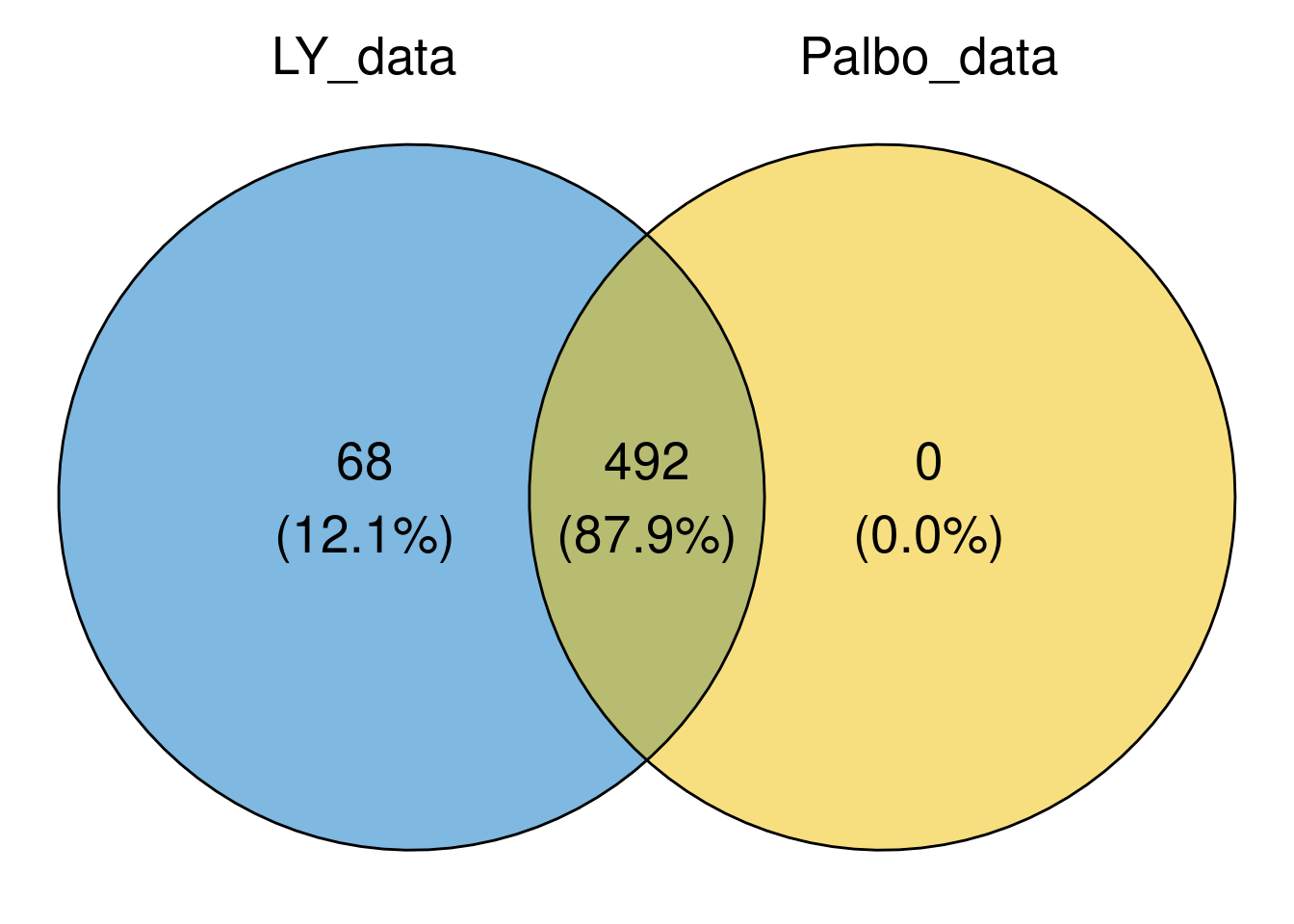
overlap of cell lines treated with LY and Palbo

list_i <- list(LY_data = LY_data$cell_line, 
               Palbo_data = Palbo_data$cell_line
)
     
LY_Palbo_overlap <- calculate.overlap(x = list_i)

For most cell lines, the IC50 value is avaialble for both LY and Palbo.

ggvenn(
  list_i, 
  fill_color = c("#0073C2FF", "#EFC000FF", "#868686FF"),
  stroke_size = 0.5, set_name_size = 7, text_size = 7
  )

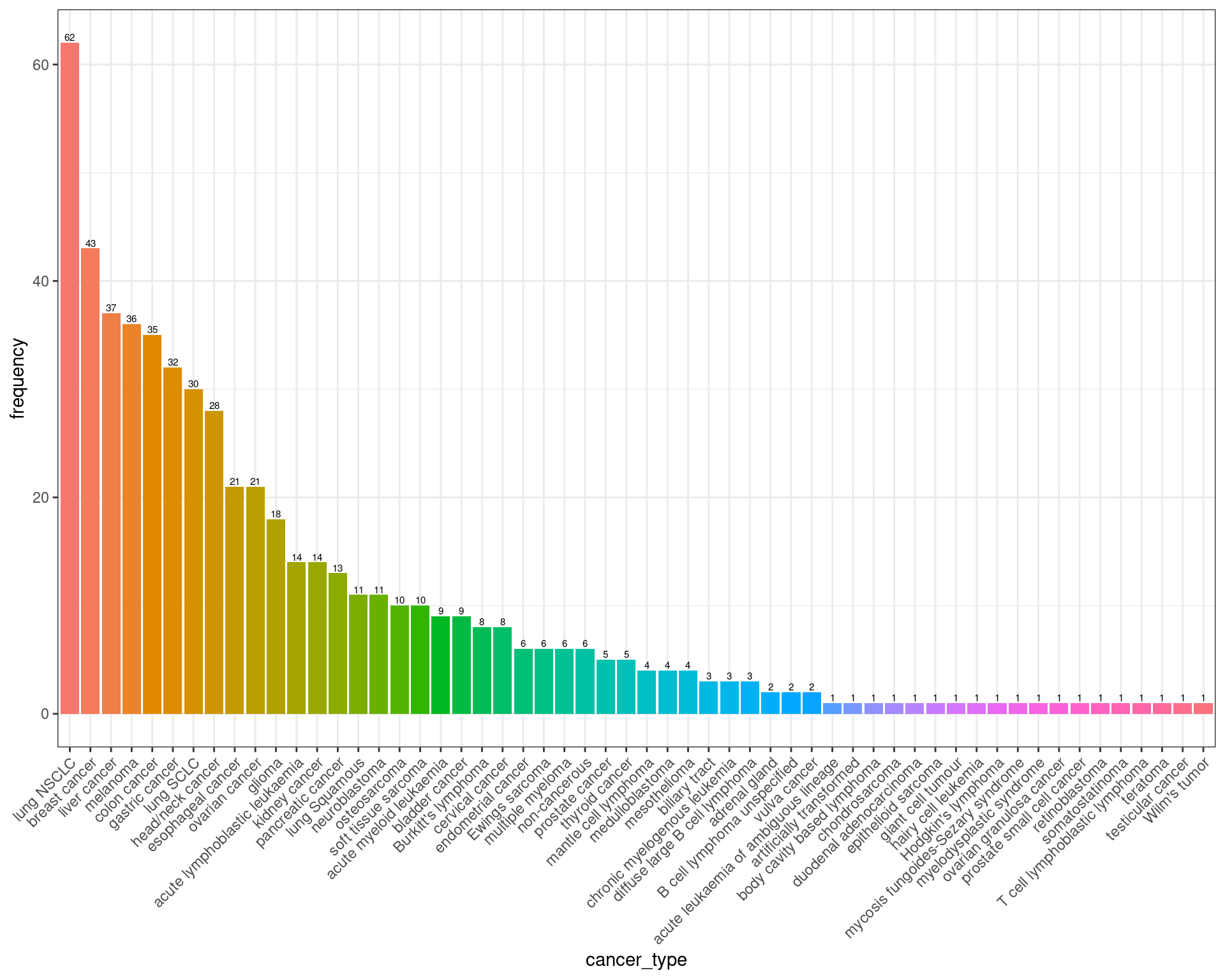
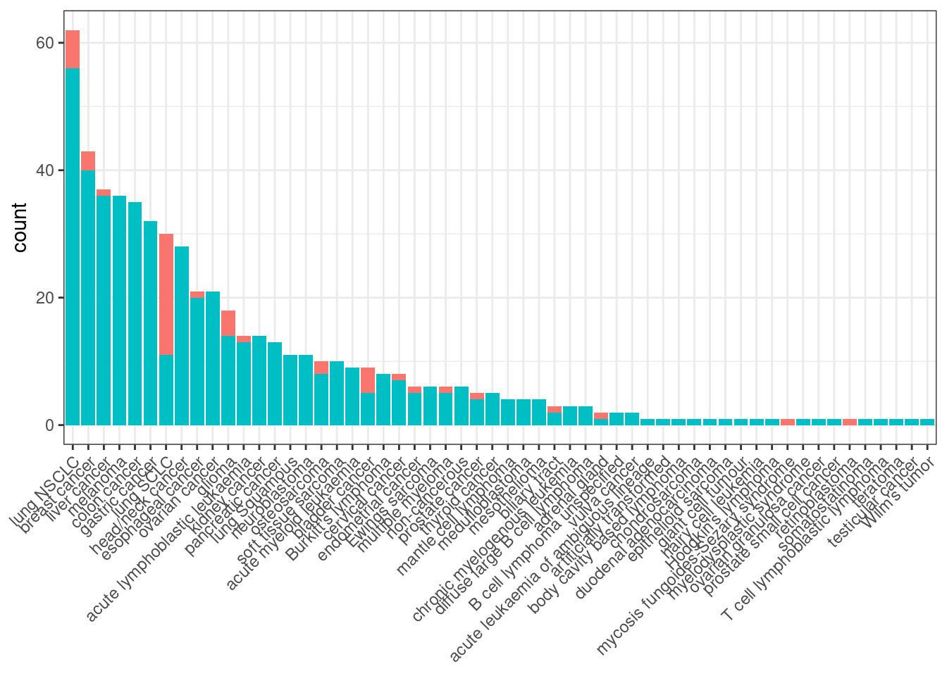
cancer type summary

cancer_type_df <- combined_data$cancer_type_LY %>% table %>% sort(decreasing = TRUE) %>% data.frame
colnames(cancer_type_df) <- c("cancer_type", "frequency")

cancer_type_df %>% ggplot(aes(x = cancer_type, y = frequency, fill = cancer_type)) + 
  geom_bar(stat = "identity") +
  geom_text(aes(label=frequency), position=position_dodge(width=0.9), vjust=-0.25, size = 2) +
  theme_bw() + 
  theme(legend.position = "none", legend.title = element_blank() ,axis.text.x = element_text(angle = 45, hjust = 1))

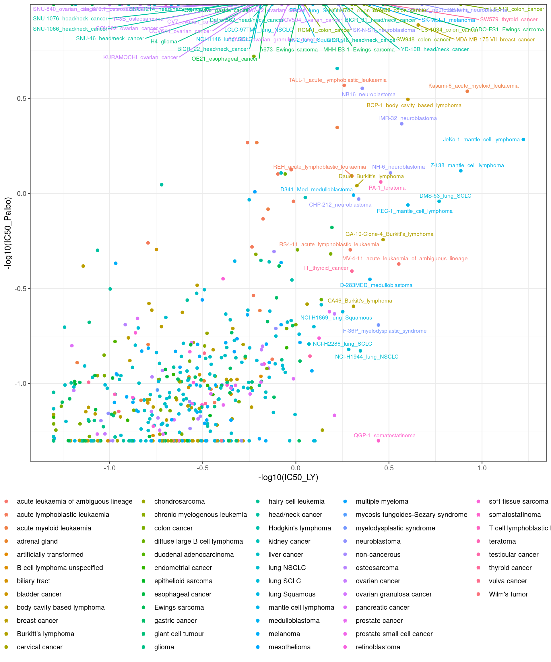
IC50 summary

cellline_i <- c(combined_data %>% dplyr::arrange(IC50_LY) %>% .$cell_line %>% head(n=40), 
                combined_data %>% dplyr::arrange(IC50_Palbo) %>% .$cell_line %>% head(n=40)) %>% unique

combined_data <- combined_data %>% unite(plot_name, cell_line, cancer_type_LY, remove = FALSE)
combined_data$plot_name <- combined_data$plot_name %>% gsub(" ", "_", .)

combined_data %>% ggplot(aes(x = -log10(IC50_LY), y = -log10(IC50_Palbo), col = cancer_type_LY)) + 
  geom_point() +
  geom_text_repel(data = combined_data %>% filter(cell_line %in% cellline_i), aes(label = plot_name), size = 2.5) + 
  theme_bw() + 
  theme(legend.position = "bottom", legend.title = element_blank())

RB mutatant status by cancer type

RB_mutant_df <- combined_data %>% 
  dplyr::group_by(cancer_type_LY, RB1_status_LY) %>% 
  summarise(count = n())

## `summarise()` has grouped output by 'cancer_type_LY'. You can override using
## the `.groups` argument.

RB_mutant_df$cancer_type_LY <- factor(RB_mutant_df$cancer_type_LY, levels = cancer_order)

#RB_mutant_df %>% head
RB_mutant_df$count %>% max()

RB_mutant_df %>% 
  ggplot(aes(x = RB1_status_LY, y = count)) + 
  geom_bar(stat= "identity") + 
  ylim(c(0, 65)) +
  facet_wrap( . ~ cancer_type_LY) +
  geom_text(aes(label=count), position=position_dodge(width=0.9), vjust=-0.25, size = 2) +
  theme_bw()

RB_mutant_df %>% 
  ggplot(aes(x = cancer_type_LY, y = count, fill = RB1_status_LY)) + 
  #geom_bar(stat=stat_count) +
  geom_bar(stat='identity') + 
  #ylim(c(0, 65)) +
  #facet_wrap( . ~ cancer_type_LY) +
  #geom_text(aes(label=count), position=position_dodge(width=0.9), vjust=-0.25, size = 2) +
  theme_bw() +
  theme(legend.position = "none", axis.title.x = element_blank() ,axis.text.x = element_text(angle = 45, hjust = 1))

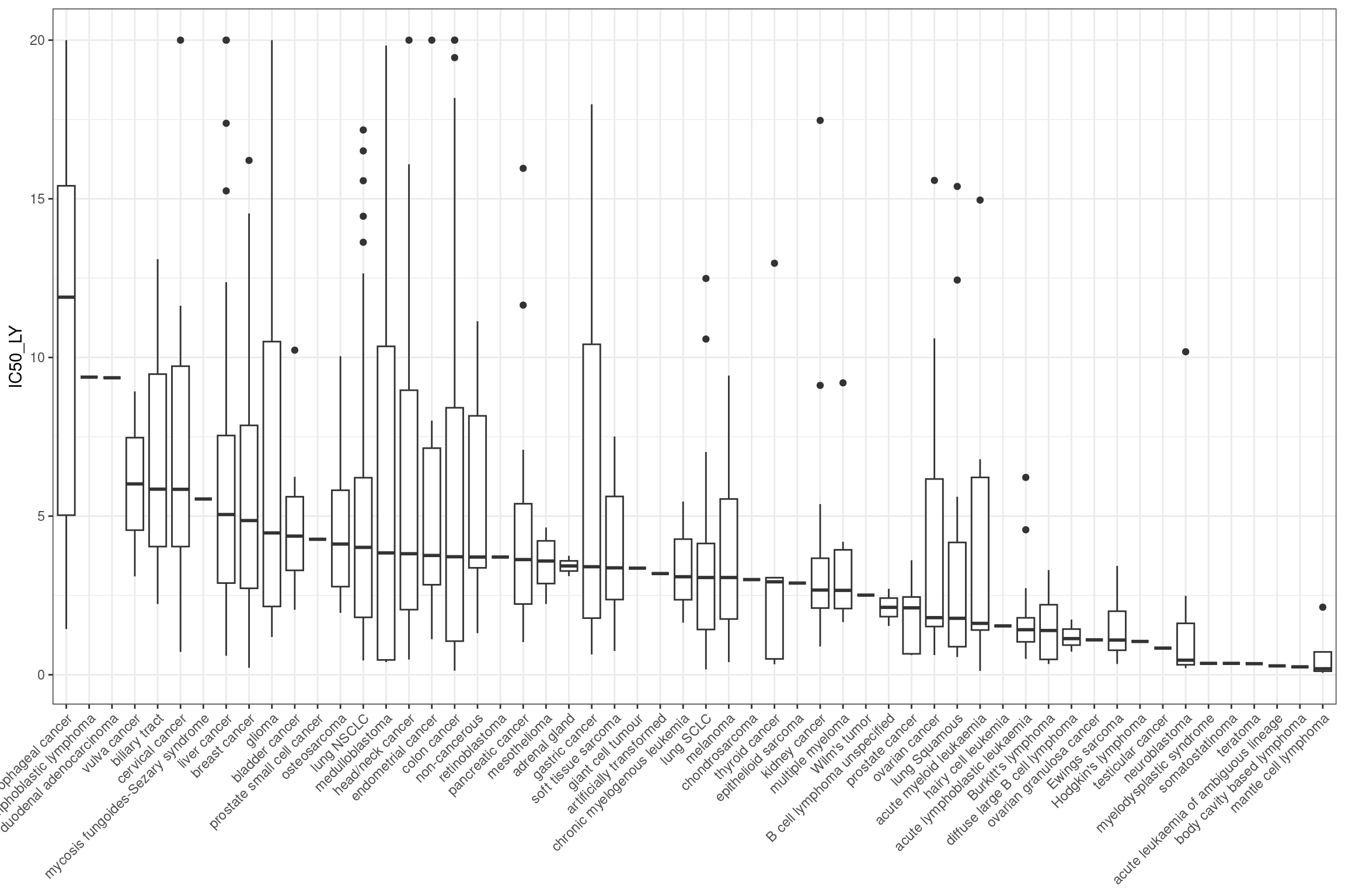
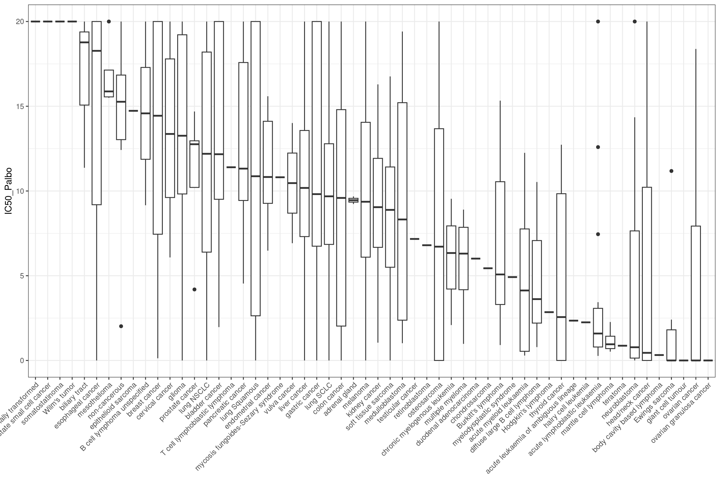
which cancer type responds the best

combined_data %>% 
  ggplot(aes(y = IC50_LY,  x = fct_reorder(cancer_type_LY, IC50_LY, .desc	
 = TRUE))) + 
  geom_boxplot() +
  theme_bw() + 
  theme(legend.position = "none", axis.title.x = element_blank() ,axis.text.x = element_text(angle = 45, hjust = 1))

combined_data %>% 
  ggplot(aes(y = IC50_Palbo,  x = fct_reorder(cancer_type_LY, IC50_Palbo, .desc	
 = TRUE))) + 
  geom_boxplot() +
  theme_bw() + 
  theme(legend.position = "none", axis.title.x = element_blank() ,axis.text.x = element_text(angle = 45, hjust = 1))

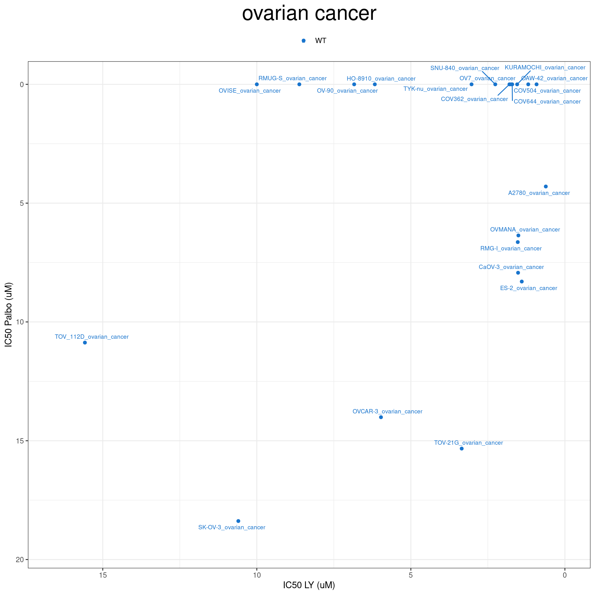
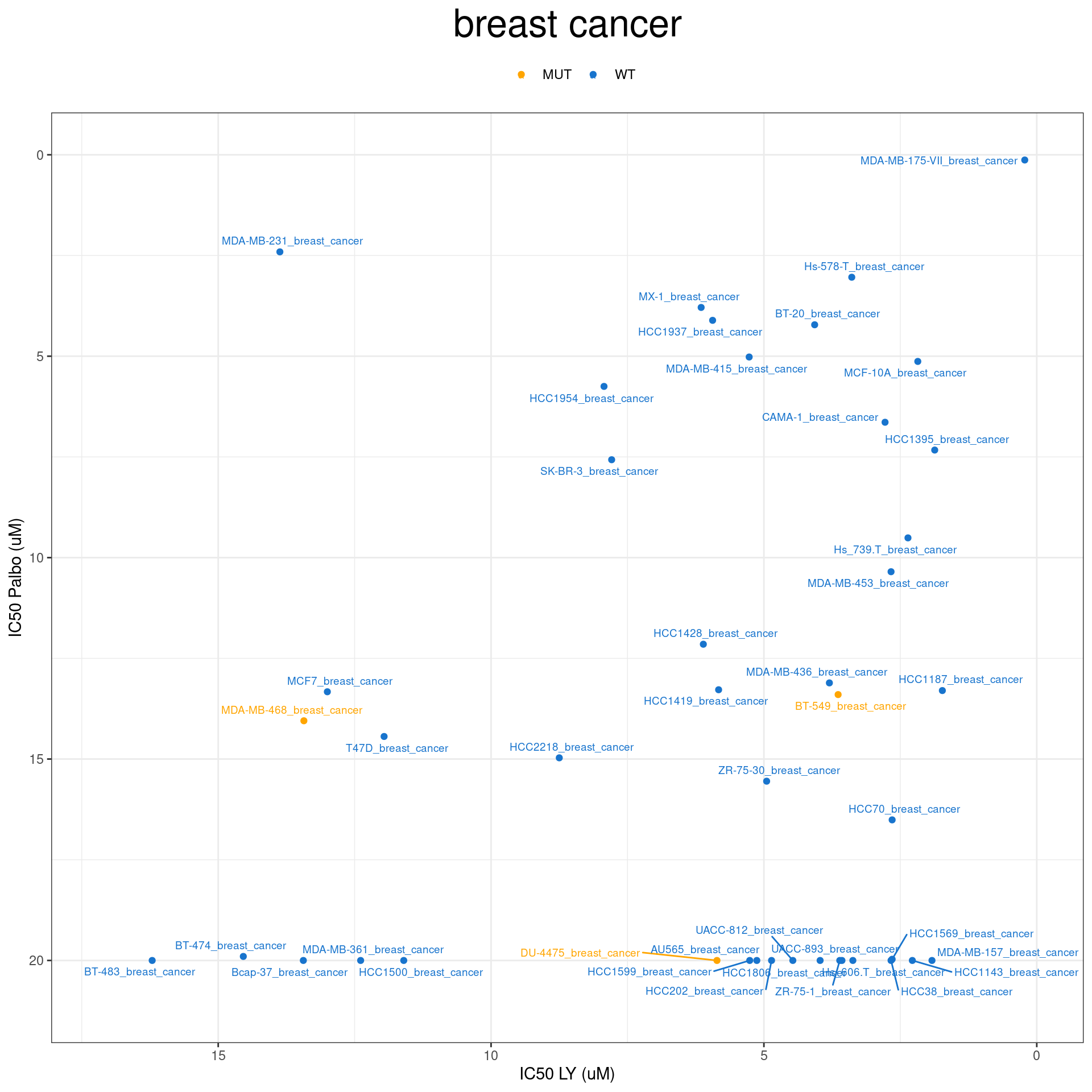
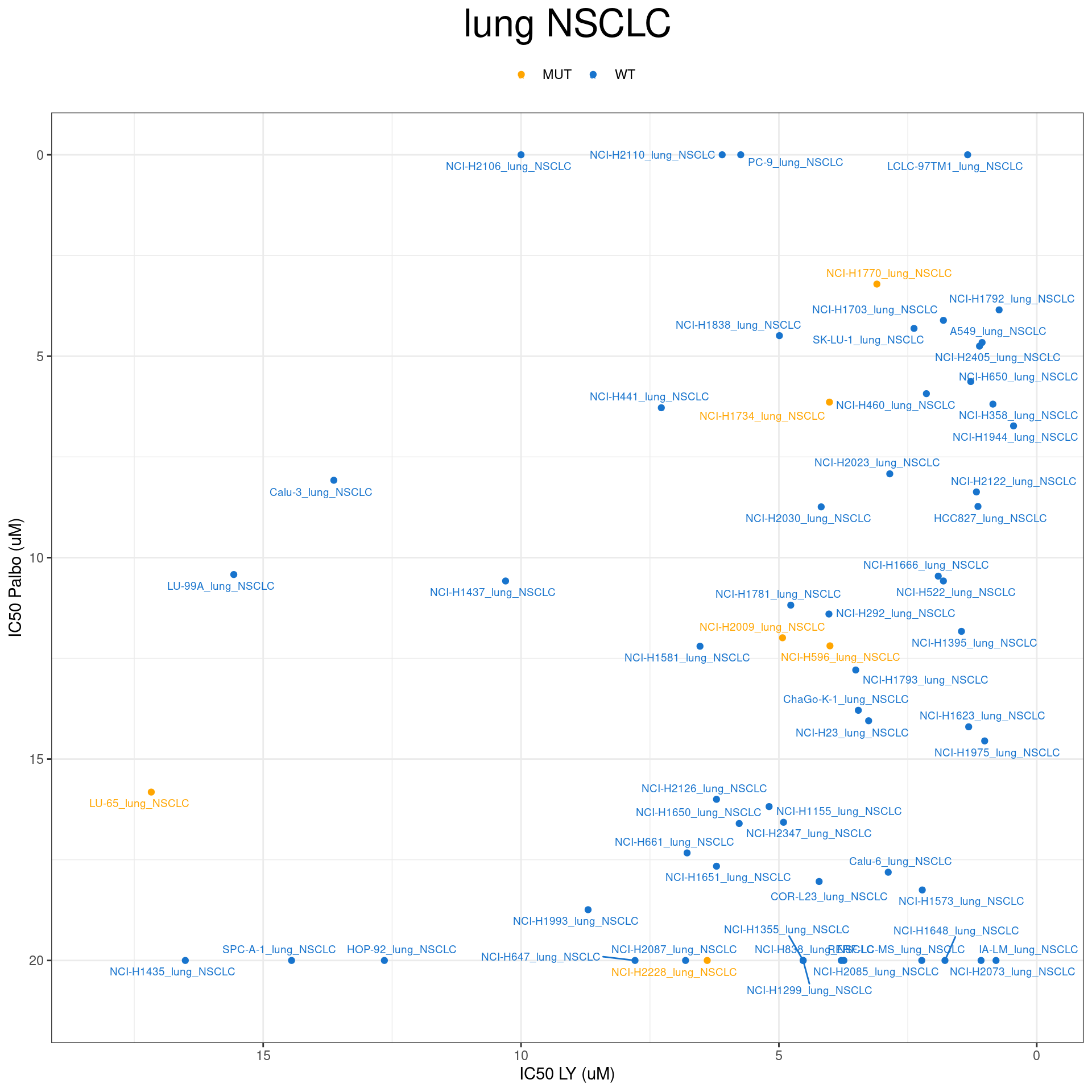
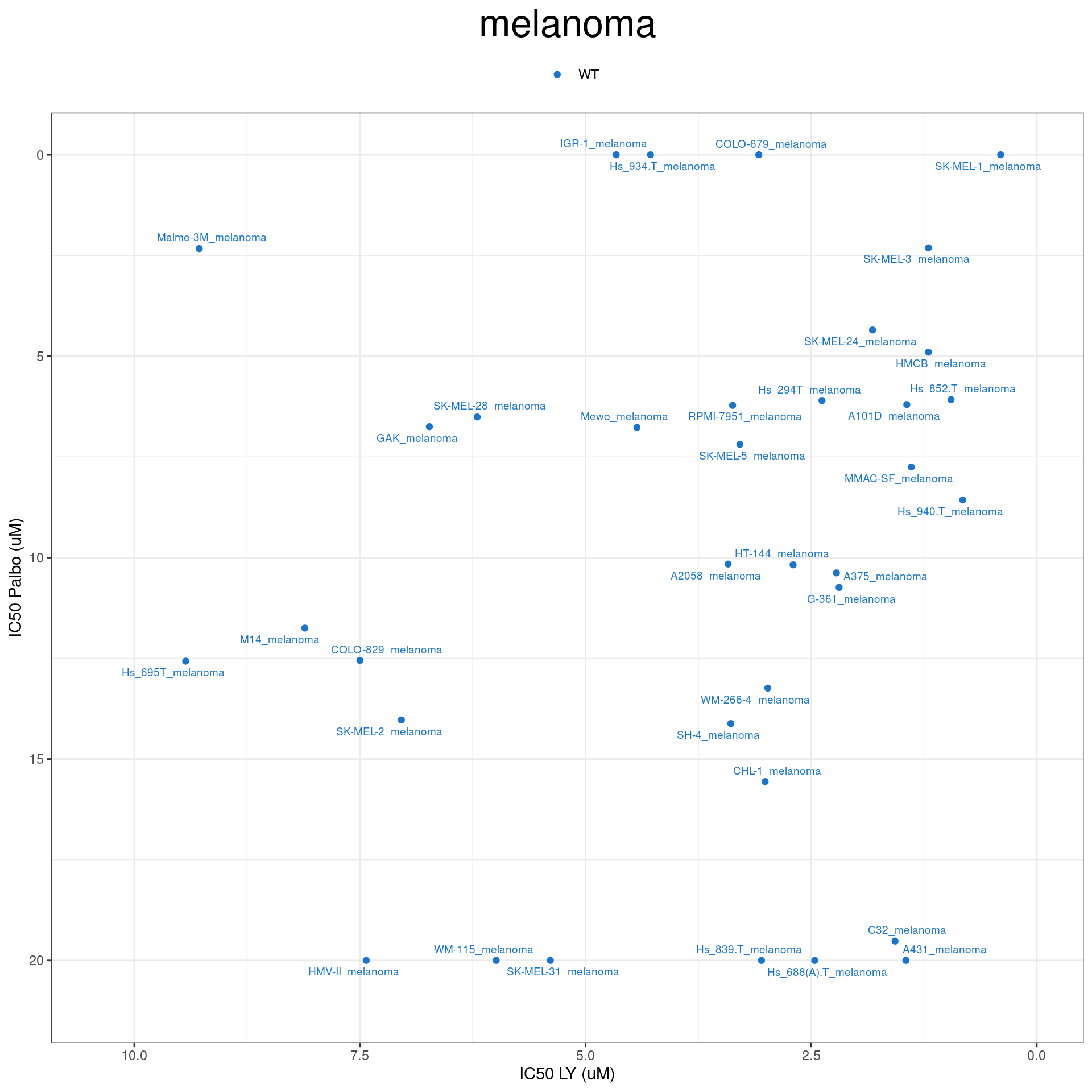
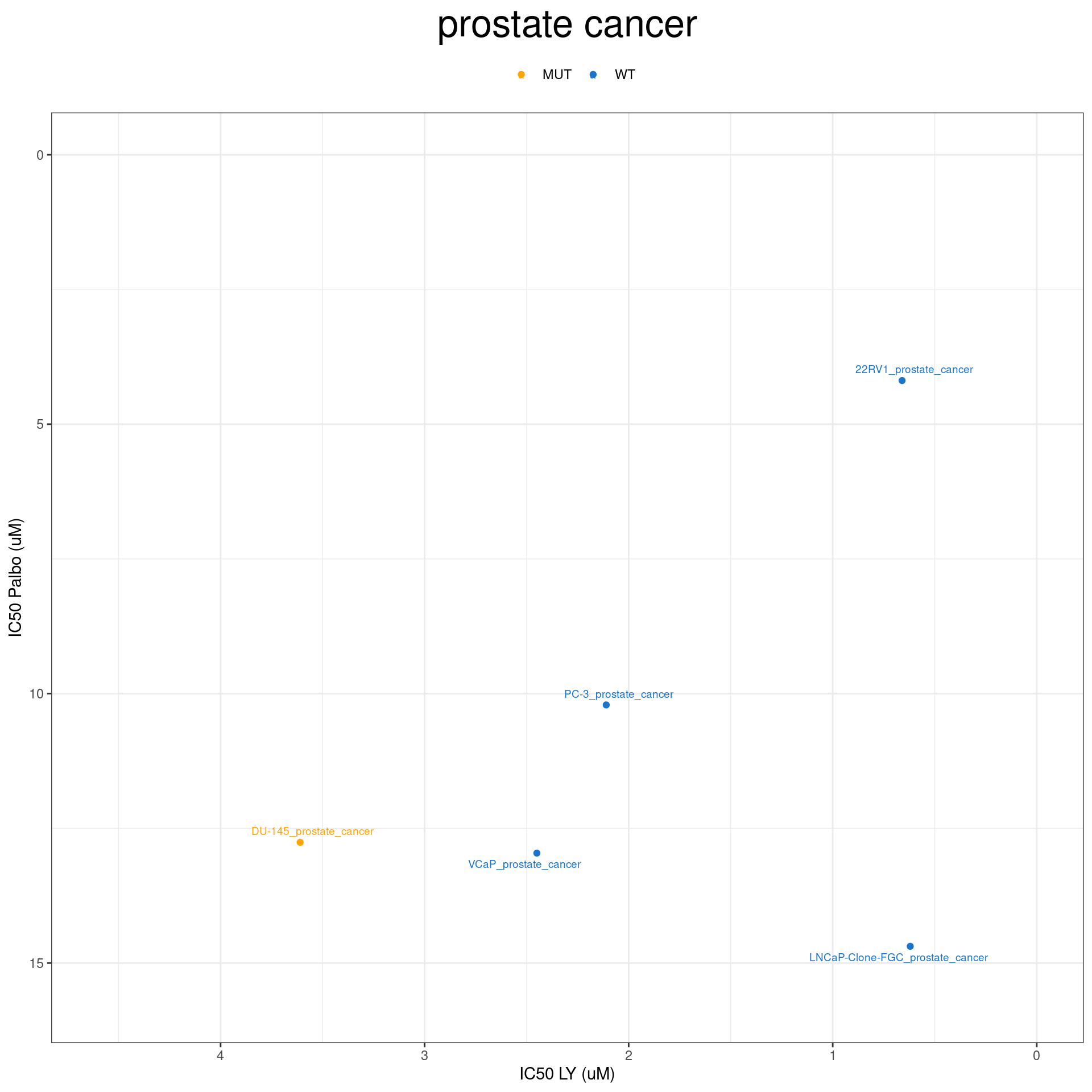
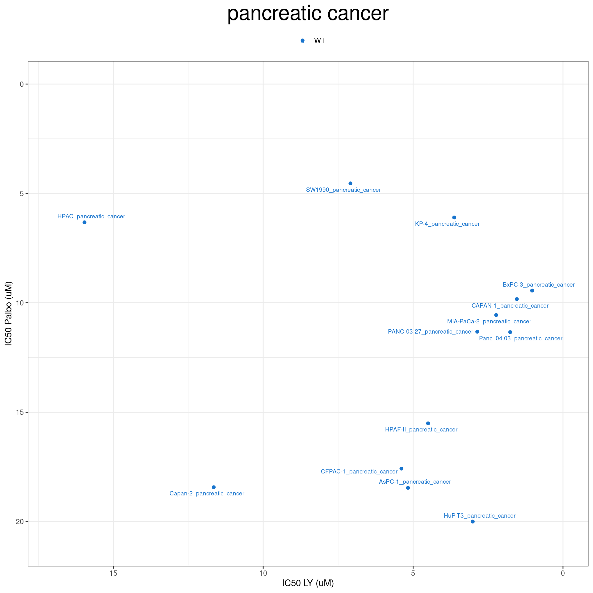
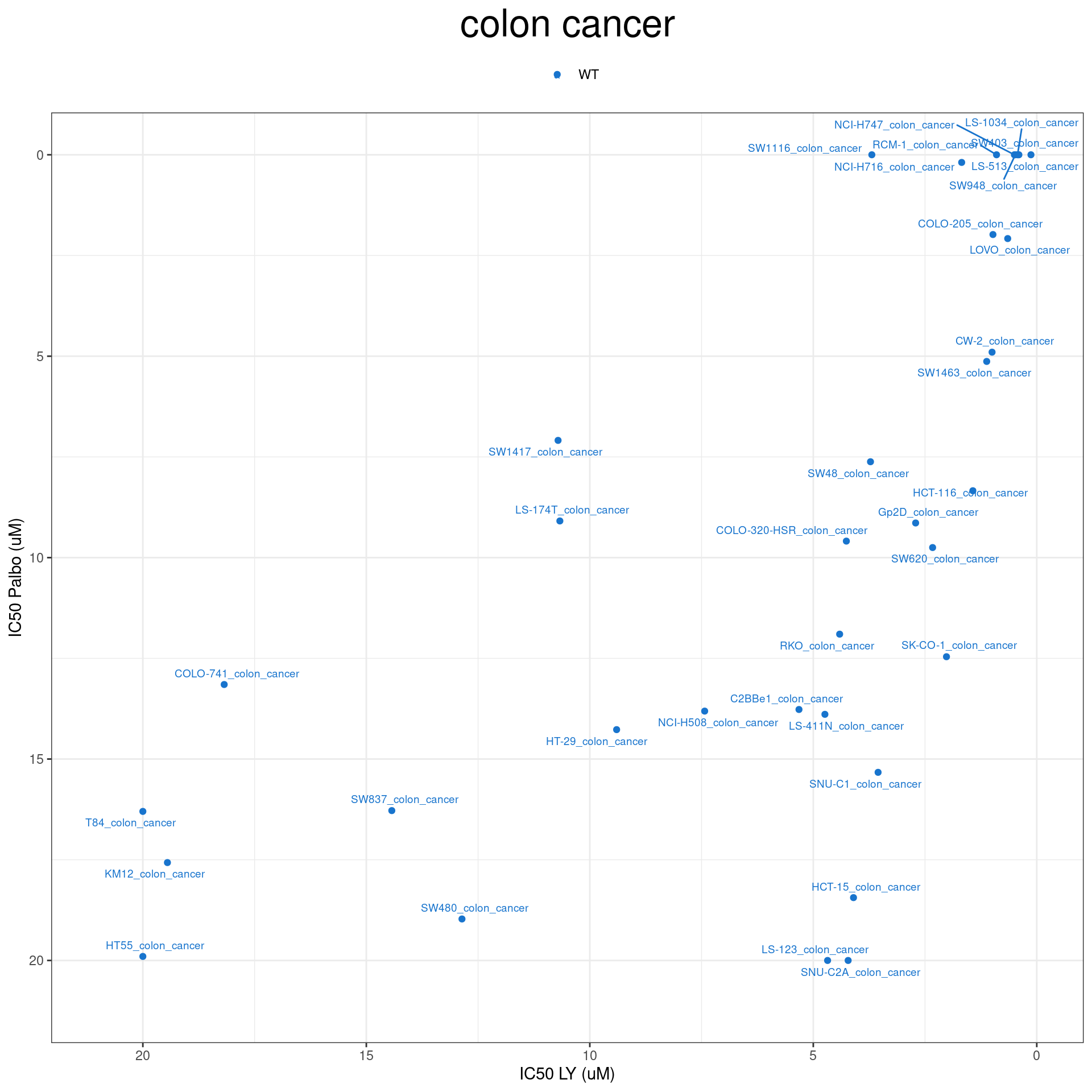
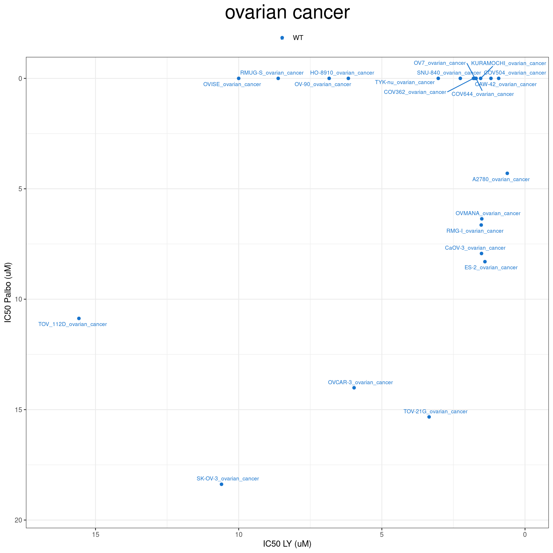
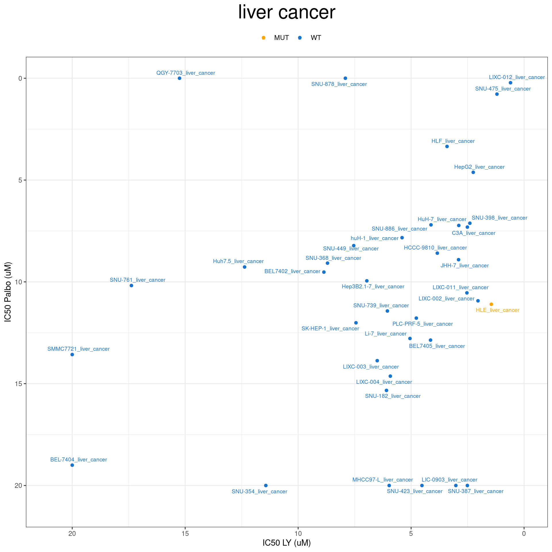
plot IC50 according to cancer type

combined_data$RB1_status_LY

RB1_col = c("WT" = "Dodgerblue3", "MUT" = "orange")

plot_IC50 <- function(type){
  temp_df <- combined_data %>% filter(cancer_type_LY == type)

  max_x = temp_df$IC50_LY %>% max %>% round(digits = 1) + 1
  max_y = temp_df$IC50_Palbo %>%  max(na.rm= TRUE) %>% round(digits = 1) +1

  temp_df %>% 
    ggplot(aes(x = IC50_LY, y = IC50_Palbo, col = RB1_status_LY)) + 
    geom_point() +
    geom_text_repel(data = temp_df, aes(label = plot_name), size = 2.5) + 
    scale_color_manual(values  = RB1_col) +
    ggtitle(type) +
    labs(x = "IC50 LY (uM)", y = "IC50 Palbo (uM)") +
    ylim(max_y, 0) +
    xlim(max_x, 0) +
    theme_bw() + 
    theme(legend.position = "top", legend.title = element_blank(), plot.title = element_text(hjust = 0.5, size=25))
  }